TAPAS Tutorial 5: Quantification

In this tutorial we will learn some basic analysis functions of TAPAS. We will learn how to use the measurement module. Please check you understand the basics of TAPAS Input/Output.

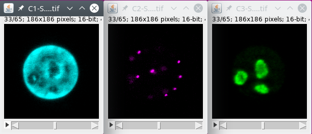
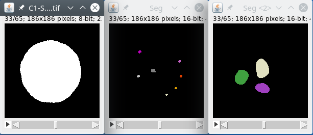
In this tutorial we will use FISH (Fluorescent In Situ Hybridization) data with labeling for the nucleus, some spots and some chromatin regions. The data can be downloaded from here.

Preparing the data : filtering and segmentation

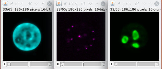
We will first filter the data to reduce the noise, and then extract the different structures.

Basically we will first filter the signal.

Then we binarize the data.

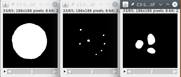
Finally, we detect the structures inside the image.

The nucleus

We will first filter the nucleus signal by using the module filters, with large radii to homogenize the signal inside the nucleus. We will then use the module autoThreshold to binarize the data. We will then label the binary image to detect the objects inside the image, we expect only one object, the nucleus, but there may be some small noise parts in the background, we will remove this part by using the module biggest that will detect the biggest object, the nucleus, and get rid of smaller parts. Finally, we will output the labeled nucleus image back to the Omero database or files.

    // input first channel
    process:input
    channel:1

    // filter nucleus
    process:filters
    radxy:4
    radz:2

    // threshold nucleus
    process:autoThreshold
    method:Triangle

    // label nucleus and keep biggest object 
    // in case small parts are segmented too
    process:label
    process:biggest

    // save resulting image
    process:output
    image:?image?-nucleus

The spots

We will first filter the spots signal by using the module filters, with small radii to reduce the noise, if we use a large radius we may lose the spots signal that are quite small. We will then use the module autoThreshold to binarize the data. We will then label the binary image to detect the objects inside the image. Finally, we will output the labeled spots image back to the Omero database or files.

    // input second channel
    process:input
    channel:2

    // filter spots
    process:filters
    radxy:2
    radz:1

    // threshold spots
    process:autoThreshold
    method:Otsu

    // label spots
    process:label
    minVolume:10

    // save results
    process:output
    image:?image?-spots

The regions

We will first filter the regions signal by using the module filters, with large radii to reduce the noise and homogenize the signal inside the regions. We will then use the module autoThreshold to binarize the data. We will then label the binary image to detect the objects inside the image. Finally, we will output the labeled regions image back to the Omero database or files.

    // input third channel
    process:input
    channel:3

    // filter regions
    process:filters
    radxy:4
    radz:2

    // threshold regions
    process:autoThreshold
    method:Otsu

    // label regions
    process:label
    minVolume:100

    // save results
    process:output
    image:?image?-regions

Quantifying the signal into objects

To quantifying signal inside objects, we will need two images, a labeled image with the objects and a signal image. If we want to quantify the nucleus signal inside the nucleus, we need the signal to be quantified, the nucleus raw signal, and the image containing the objects, the labeled image we created in the previous section.

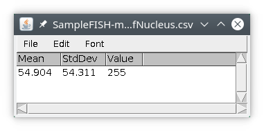
We will first input the nucleus raw data from the original image and save it locally. We will then input the nucleus labeled image. From this labeled image, we will quantify the signal coming from the locally saved image and, save the results locally also, using the module quantif. In this example we will compute the average signal intensity and the standard deviation other available statistics are min, max and sum You can also get the value at the center of the object. We will then attach the results file to the original image, either in Omero or on files.

    // open raw data for nucleus
    // and save it locally 
    // in the home directory
    // as temporary file
    process:input
    channel:1
    process:save
    dir:?home?
    file:?image?-rawNucleus

    // open labeled nucleus
    // and perform signal quantification
    process:input
    image:?image?-nucleus
    // Signal quantification
    // load signal image
    // save results locally
    process:quantif
    dirRaw:?home?
    fileRaw:?image?-rawNucleus
    list:mean,sd
    dir:?home?
    file:?image?-quantifNucleus.csv

    // attach result to image
    // and delete temporary files
    process:attach
    dir:?home?
    file:?image?-quantifNucleus.csv
    process:deleteList
    dir:?home?
    list:?image?-quantifNucleus.csv,?image?-nucleus

We will then obtain a results table with only one row, with the results of quantification (note here mean and sd have quite similar values). The column value is simply the value of the object in the labeled image.

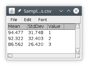
We can do the same for the chromatin regions.

    // open raw regions
    // and save it locally 
    // as temporary file
    process:input
    channel:3
    process:save
    dir:?home?
    file:?image?-rawRegions

    // open labeled regions
    // and perform signal quantification
    process:input
    image:?image?-regions
    // Signal quantification
    // load signal image
    // save results locally
    process:quantif
    dirRaw:?home?
    fileRaw:?image?-rawRegions
    list:mean,sd
    dir:?home?
    file:?image?-quantifRegions.csv

    // attach result to image
    // and delete temporary files
    process:attach
    dir:?home?
    file:?image?-quantifRegions.csv
    process:deleteList
    dir:?home?
    list:?image?-quantifRegions.csv,?image?-regions

We will then obtain a results table with three rows, with the results of quantification. The column value is simply the value (id) of the object in the labeled image.

Numbering objects

Numbering simply consists of counting the number of objects inside bigger objects, in our case we will count the number of spots inside the nucleus. We need two labeled images, one for the spots and one for the nucleus.

First we will input the spots labeled image that we created previously and save it locally. We will then input the nucleus labeled image and use the module number to count the number of spots inside the nucleus. The results file will be saved locally, we will then attach it to the original image.

    // open labeled spots
    // and save it locally 
    // as temporary file
    process:input
    image:?name?-spots
    process:save
    dir:?home?
    file:?image?-labelSpots

    // open labeled nucleus
    // and perform numbering
    process:input
    image:?image?-nucleus
    process:number
    dirLabel:?home?
    fileLabel:?image?-labelSpots
    dir:?home?
    file:?image?-numberNucleusSpots.csv

    // attach result to image
    // and delete temporary files
    process:attach
    dir:?home?
    file:?image?-numberNucleusSpots.csv
    process:deleteList
    dir:?home?
    list:?image?-numberNucleusSpots.csv,?image?-spots

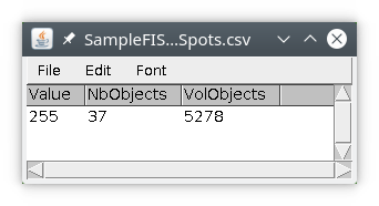
We obtain a results table with one row, indicating the number of objects, here 3, and the volume (in pixels) occupied by these object inside the nucleus object.